Chapter 7 Categorical predictors and interactions

By the end of this chapter you will:

Understand how to use R factors, which automatically deal with fiddly aspects of using categorical predictors in statistical models.
Be able to relate R output to what is going on behind the scenes, i.e., coding of a category with $n$-levels in terms of $n-1$ binary 0/1 predictors.
See how R does interactions effects (the * and : operators).

The lovely thing about the topics covered in this chapter is that they all transfer to every other model, e.g., logistic regression and other generalised linear models, multilevel models, and a huge number of models which you may encounter in future.

7.1 Before we begin

We are going to persist with the prestige dataset another time. (Last chapter, promise.) You could continue on the end of last week’s Markdown file or make a new one.

Ensure these handy packages are installed (you will only have to do that once) and included:

library(car)
library(tidyverse)

7.2 The dataset

For ease of reference. Each row describes an occupation and aggregated data about that occupation (in 1970s Canada).

Variable name	Description
occ	Occupation
education	Average years of education for people in the job
income	Average income in dollars
women	Percentage of women in occupation
prestige	A Pineo-Porter prestige score for the occupation with a possible range of 0-100 (higher = more prestigious)
type	“bc” = blue collar “wc” = white collar “prof” = professional, managerial, or technical

Read it in:

dat <- read.csv("prestige.csv")

This week we will explore whether there are mean differences in prestige between the three types of profession: blue collar, white collar, and professional.

7.3 Factors

R has a special kind of object called a factor for representing categorical variables in statistical models. Ensure that R “knows” that you want to treat type as a factor by doing the following:

dat$type <- factor(dat$type)

You can check whether a variable is a factor by doing:

is.factor(dat$type)

## [1] TRUE

Here’s a variable that isn’t:

is.factor(dat$prestige)

## [1] FALSE

It’s numeric…

is.numeric(dat$prestige)

## [1] TRUE

You can also look up the “class” of a variable:

class(dat$type)

## [1] "factor"

You can check the levels of a factor by using the levels function:

levels(dat$type)

## [1] "bc"   "prof" "wc"

The order is alphabetical by default and can easily be changed.

The levels function only works for factors:

levels(dat$prestige)

## NULL

7.4 Visualising the data

(I go through this in some detail, for information. Feel free to skip over it on first reading.)

We will be exploring whether there are differences in a continuous variable (prestige) between levels of a categorical variable (type).

A traditional visualisation for this genre of comparison is the bar plot, with either standard error of the mean (SE mean) or standard deviation (SD) error bars.

These days, the recommendation is to look at the raw data before reducing it to means, for instance with a jitter plot.

set.seed(100) # Optional
dat %>%
  ggplot(aes(type, prestige, colour = type)) +
  geom_jitter(height = 0,
              width = .1,
              show.legend = FALSE) +
  ylim(0,100)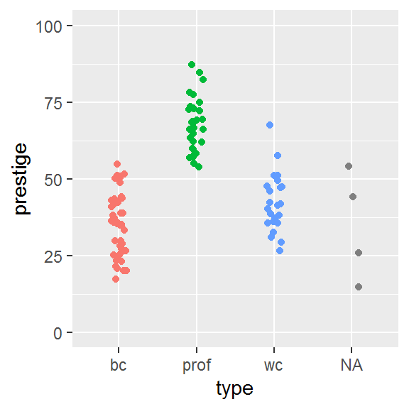

We can see 4 observations in an “NA” category. Those are missing data, i.e., values in the dataset which have not been assigned a type.

dat %>%
  filter(is.na(type))

##           occ education income women prestige type
## 1    athletes     11.44   8206  8.13     54.1 <NA>
## 2    newsboys      9.62    918  7.00     14.8 <NA>
## 3 babysitters      9.46    611 96.53     25.9 <NA>
## 4     farmers      6.84   3643  3.60     44.1 <NA>

Also note that I have fixed the y-axis scale so that it covers the theoretical range of the prestige measure (0-100) rather than only the values present in the data.

Here is how to make the traditional bar plot. First calculate the means and standard error of the means for each group. The standard error is calculated as

\[ \frac{\mathit{SD}}{\sqrt{N}} \] where $N$ is the number of observations. R has a function called sqrt for calculating the square root:

sqrt(4)

## [1] 2

We use group_by as before to ask tidyverse to group observations by type of occupation, and then summarise the data. The n function simply counts the number of observations, which will also be calculated per group following the group_by.

dat_means <- dat %>%
  group_by(type) %>%
  summarise(mean = mean(prestige),
            SD   = sd(prestige),
            SE   = SD/sqrt(n()),
            n    = n())
dat_means

## # A tibble: 4 x 5
##   type   mean    SD    SE     n
##   <fct> <dbl> <dbl> <dbl> <int>
## 1 bc     35.5 10.0   1.51    44
## 2 prof   67.8  8.68  1.56    31
## 3 wc     42.2  9.52  1.98    23
## 4 <NA>   34.7 17.7   8.84     4

Here is how I went about plotting these values.

I began by plotting the means:

dat_means %>%
  ggplot(aes(type, mean)) +
  geom_bar(stat = "identity")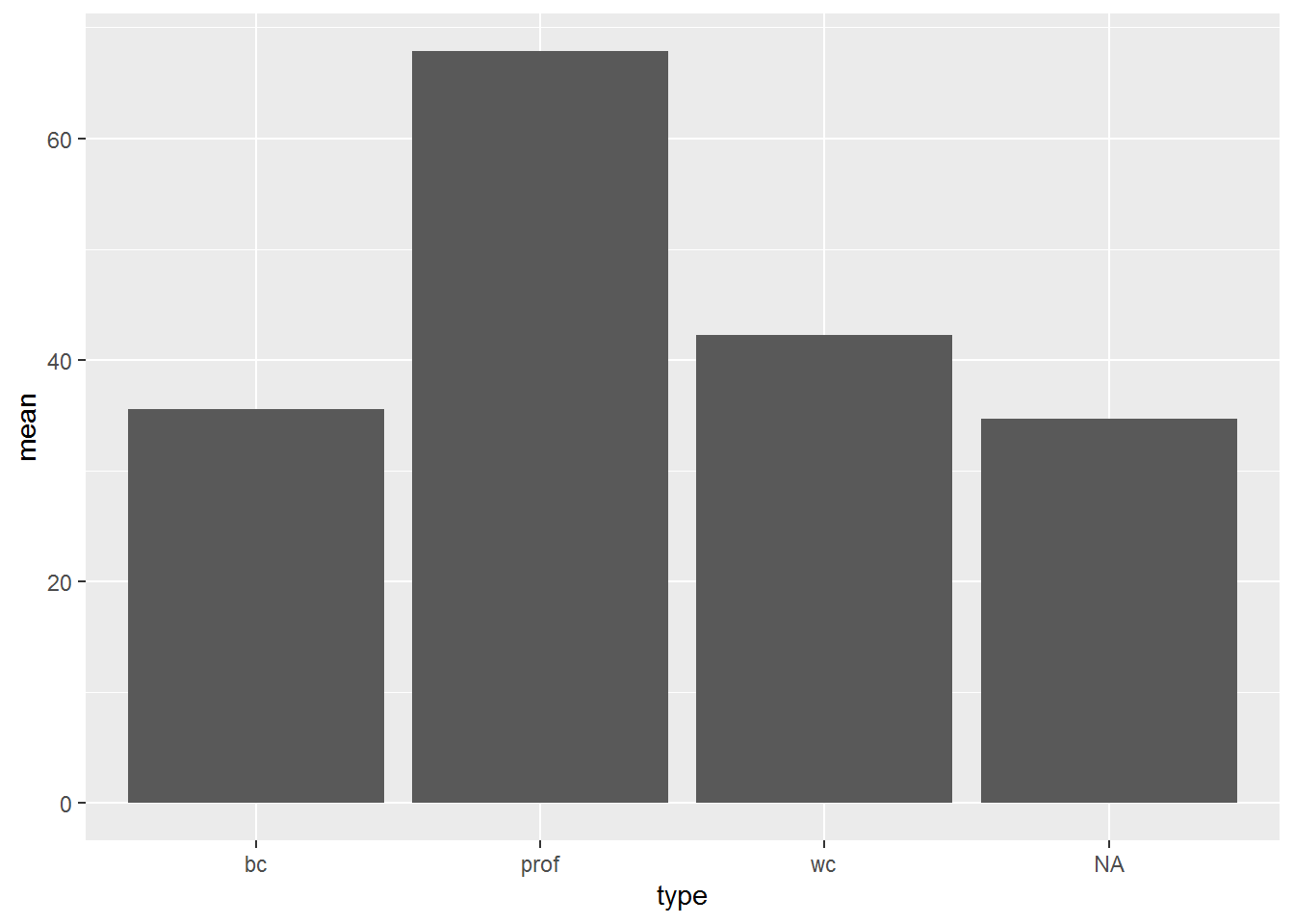

Then I added error bars:

dat_means %>%
  ggplot(aes(type, mean)) +
  geom_bar(stat = "identity") +
  geom_errorbar(aes(ymin = mean - SE,
                    ymax = mean + SE))

Following this, I fiddled around for fifteen minutes, wishing I had just looked up a bar plot I had made previously… (The lesson here is, build a stash of example R code you can quickly find, adapt, and reuse.)

dat_means %>%
  filter(!is.na(type)) %>%
  ggplot(aes(type, mean, fill = type)) +
  geom_bar(stat = "identity", show.legend = F) +
  geom_errorbar(aes(ymin = mean - SE,
                    ymax = mean + SE), width = 1/4) +
  xlab("Occupation type") +
  ylab("Mean prestige") +
  ylim(0, 100) +
  theme_classic()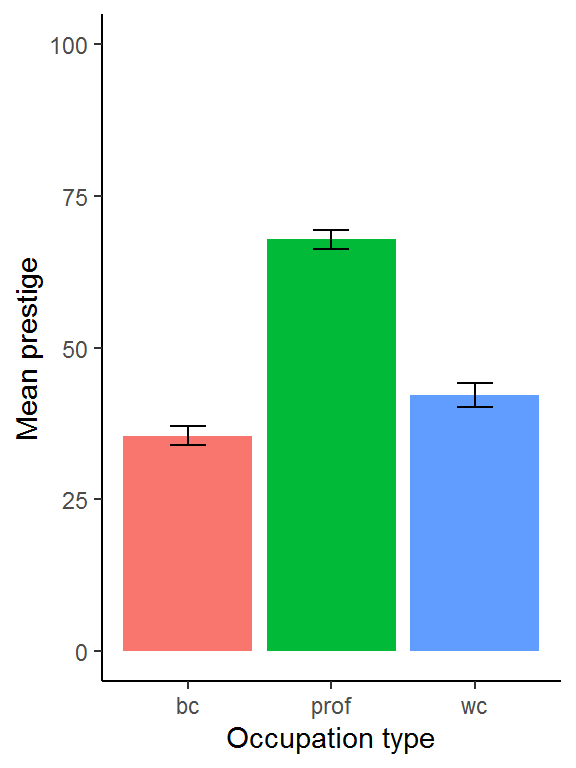

You might want to add standard deviation bars instead:

dat_means %>%
  filter(!is.na(type)) %>%
  ggplot(aes(type, mean, fill = type)) +
  geom_bar(stat = "identity", show.legend = F) +
  geom_errorbar(aes(ymin = mean - SD,
                    ymax = mean + SD), width = 1/4) +
  xlab("Occupation type") +
  ylab("Mean prestige") +
  ylim(0, 100) + 
  theme_classic()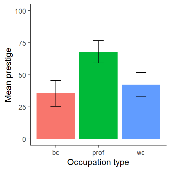

You might also want less vibrant colours, e.g., if you wish to include the graph in a publication:

dat_means %>%
  filter(!is.na(type)) %>%
  ggplot(aes(type, mean)) +
  geom_bar(stat = "identity", fill = "grey") +
  geom_errorbar(aes(ymin = mean - SD,
                    ymax = mean + SD), width = 1/4) +
  xlab("Occupation type") +
  ylab("Mean prestige") +
  ylim(0,100) +
  theme_classic()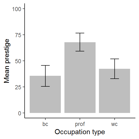

These are the chunk options I used to change the dimensions of the figure, which might be handy to know about too (they go at the top of the chunk):

{r fig.height=3, fig.width=3}

7.5 The punchline: occupation type does predict prestige

This is where we are heading.

First, select the variables you want to model and remove missing values:

dat_no_NAs <- dat %>%
  select(occ, prestige, type) %>%
  na.omit()

We could just have removed missing variables from the whole dataset – it would have worked for the prestige dataset since there are only four missing values and they are all in one variable. However, for larger datasets doing so might easily wipe out everything! For more on handling missing data correctly, try the book by van Buuren (2018).

Now, fit an intercept-only model and compare it with a model which has type as a predictor. R will automatically do something sensible with type since it knows that it is a factor.

intercept_only <- lm(prestige ~ 1, data = dat_no_NAs)
type_mod       <- lm(prestige ~ type, data = dat_no_NAs)
                             # (the 1 is implicit)

anova(intercept_only, type_mod)

## Analysis of Variance Table
## 
## Model 1: prestige ~ 1
## Model 2: prestige ~ type
##   Res.Df     RSS Df Sum of Sq      F    Pr(>F)    
## 1     97 28346.9                                  
## 2     95  8571.3  2     19776 109.59 < 2.2e-16 ***
## ---
## Signif. codes:  0 '***' 0.001 '**' 0.01 '*' 0.05 '.' 0.1 ' ' 1

Occupation type does indeed explain variation in prestige, $F(2,95) = 109.59$, $p < .001$.

An even easier way to do this is using car’s Anova command (uppercase A). This does not require you to fit an intercept-only model yourself and deals with multiple predictors (handy later):

type_mod <- lm(prestige ~ type, data = dat_no_NAs)
Anova(type_mod)

## Anova Table (Type II tests)
## 
## Response: prestige
##            Sum Sq Df F value    Pr(>F)    
## type      19775.6  2  109.59 < 2.2e-16 ***
## Residuals  8571.3 95                      
## ---
## Signif. codes:  0 '***' 0.001 '**' 0.01 '*' 0.05 '.' 0.1 ' ' 1

Read on to see why this has worked and also to work out which of the three occupations differ from each other in prestige…

7.6 Understanding factors in regression models

7.6.1 How are categorical variables encoded?

Let’s begin with an easier example with only two groups: blue collar and white collar occupations:

just_two <- dat %>%
  filter(type %in% c("bc","wc")) %>%
  select(occ, prestige, type)

Here are the means of prestige for both groups:

just_two %>%
  group_by(type) %>%
  summarise(mean_prestige = mean(prestige))

## # A tibble: 2 x 2
##   type  mean_prestige
##   <fct>         <dbl>
## 1 bc             35.5
## 2 wc             42.2

Next, let’s fit a regression model, predicting prestige from occupation type:

easier <- lm(prestige ~ type, data = just_two)
summary(easier)

## 
## Call:
## lm(formula = prestige ~ type, data = just_two)
## 
## Residuals:
##      Min       1Q   Median       3Q      Max 
## -18.2273  -7.0273  -0.2273   6.8227  25.2565 
## 
## Coefficients:
##             Estimate Std. Error t value Pr(>|t|)    
## (Intercept)   35.527      1.486  23.914   <2e-16 ***
## typewc         6.716      2.536   2.649   0.0101 *  
## ---
## Signif. codes:  0 '***' 0.001 '**' 0.01 '*' 0.05 '.' 0.1 ' ' 1
## 
## Residual standard error: 9.855 on 65 degrees of freedom
## Multiple R-squared:  0.09742,    Adjusted R-squared:  0.08353 
## F-statistic: 7.016 on 1 and 65 DF,  p-value: 0.01013

Note how we told lm that the predictor is type; however, the summary is displaying a slope for typewc. Curious…

7.6.1.1 Activity

Examine the estimates (the intercept and the slope for typewc) in this model and compare them with the means of the two groups. Can you see where the numbers come from?

7.6.1.2 Answer

The intercept is the same as the mean prestige for bc ($35.527$) and the slope for typewc is equal to the mean difference in prestige between the two groups: white collar minus blue collar ($42.243 - 35.527 = 6.716$).

7.6.2 How are binary (two-level) categorical predictors encoded?

First let me emphasise that you do not need to do this coding yourself; this section aims to demonstrate how the coding works, not how to carry out an analysis.

When you have a binary categorical variable (one with two levels), one level is coded as 0 and the other as 1. By default, R chooses alphabetically.

Here is something equivalent – a “hand coded” variable which is 1 for white collar occupations and 0 for blue collar:

just_two$type_wc <- as.numeric(just_two$type == "wc")

Have a look, comparing the type column with type_wc:

just_two

##                          occ prestige type type_wc
## 1              nursing aides     34.9   bc       0
## 2        medical technicians     67.5   wc       1
## 3        radio tv announcers     57.6   wc       1
## 4                secretaries     46.0   wc       1
## 5                    typists     41.9   wc       1
## 6                bookkeepers     49.4   wc       1
## 7           tellers cashiers     42.3   wc       1
## 8         computer operators     47.7   wc       1
## 9            shipping clerks     30.9   wc       1
## 10               file clerks     32.7   wc       1
## 11              receptionsts     38.7   wc       1
## 12             mail carriers     36.1   wc       1
## 13             postal clerks     37.2   wc       1
## 14       telephone operators     38.1   wc       1
## 15                collectors     29.4   wc       1
## 16           claim adjustors     51.1   wc       1
## 17             travel clerks     35.7   wc       1
## 18             office clerks     35.6   wc       1
## 19         sales supervisors     41.5   wc       1
## 20     commercial travellers     40.2   wc       1
## 21              sales clerks     26.5   wc       1
## 22 service station attendant     23.3   bc       0
## 23          insurance agents     47.3   wc       1
## 24      real estate salesmen     47.1   wc       1
## 25                    buyers     51.1   wc       1
## 26              firefighters     43.5   bc       0
## 27                 policemen     51.6   bc       0
## 28                     cooks     29.7   bc       0
## 29                bartenders     20.2   bc       0
## 30         funeral directors     54.9   bc       0
## 31                launderers     20.8   bc       0
## 32                  janitors     17.3   bc       0
## 33        elevator operators     20.1   bc       0
## 34              farm workers     21.5   bc       0
## 35      rotary well drillers     35.3   bc       0
## 36                    bakers     38.9   bc       0
## 37            slaughterers 1     25.2   bc       0
## 38            slaughterers 2     34.8   bc       0
## 39                   canners     23.2   bc       0
## 40           textile weavers     33.3   bc       0
## 41         textile labourers     28.8   bc       0
## 42           tool die makers     42.5   bc       0
## 43                machinists     44.2   bc       0
## 44       sheet metal workers     35.9   bc       0
## 45                   welders     41.8   bc       0
## 46              auto workers     35.9   bc       0
## 47          aircraft workers     43.7   bc       0
## 48        electronic workers     50.8   bc       0
## 49        radio tv repairmen     37.2   bc       0
## 50     sewing mach operators     28.2   bc       0
## 51            auto repairmen     38.1   bc       0
## 52        aircraft repairmen     50.3   bc       0
## 53        railway sectionmen     27.3   bc       0
## 54        electrical linemen     40.9   bc       0
## 55              electricians     50.2   bc       0
## 56      construction foremen     51.1   bc       0
## 57                carpenters     38.9   bc       0
## 58                    masons     36.2   bc       0
## 59            house painters     29.9   bc       0
## 60                  plumbers     42.9   bc       0
## 61    construction labourers     26.5   bc       0
## 62           train engineers     48.9   bc       0
## 63               bus drivers     35.9   bc       0
## 64              taxi drivers     25.1   bc       0
## 65              longshoremen     26.1   bc       0
## 66               typesetters     42.2   bc       0
## 67               bookbinders     35.2   bc       0

Now let’s fit a regression model with this binary 0/1 variable as a predictor:

the_binary <- lm(prestige ~ type_wc, data = just_two)
summary(the_binary)

## 
## Call:
## lm(formula = prestige ~ type_wc, data = just_two)
## 
## Residuals:
##      Min       1Q   Median       3Q      Max 
## -18.2273  -7.0273  -0.2273   6.8227  25.2565 
## 
## Coefficients:
##             Estimate Std. Error t value Pr(>|t|)    
## (Intercept)   35.527      1.486  23.914   <2e-16 ***
## type_wc        6.716      2.536   2.649   0.0101 *  
## ---
## Signif. codes:  0 '***' 0.001 '**' 0.01 '*' 0.05 '.' 0.1 ' ' 1
## 
## Residual standard error: 9.855 on 65 degrees of freedom
## Multiple R-squared:  0.09742,    Adjusted R-squared:  0.08353 
## F-statistic: 7.016 on 1 and 65 DF,  p-value: 0.01013

Again, the intercept provides the mean prestige for blue collar and the slope for type_wc gives the mean difference between blue collar and white collar. This model is mathematically identical to the one that R built using the factor variable.

A (slightly jittered) picture might help you see why this is.

set.seed(45)
just_two %>%
  ggplot(aes(type_wc,prestige)) +
  geom_jitter(width = .02, height = 0) +
  geom_abline(intercept = coef(the_binary)[1],
              slope     = coef(the_binary)[2])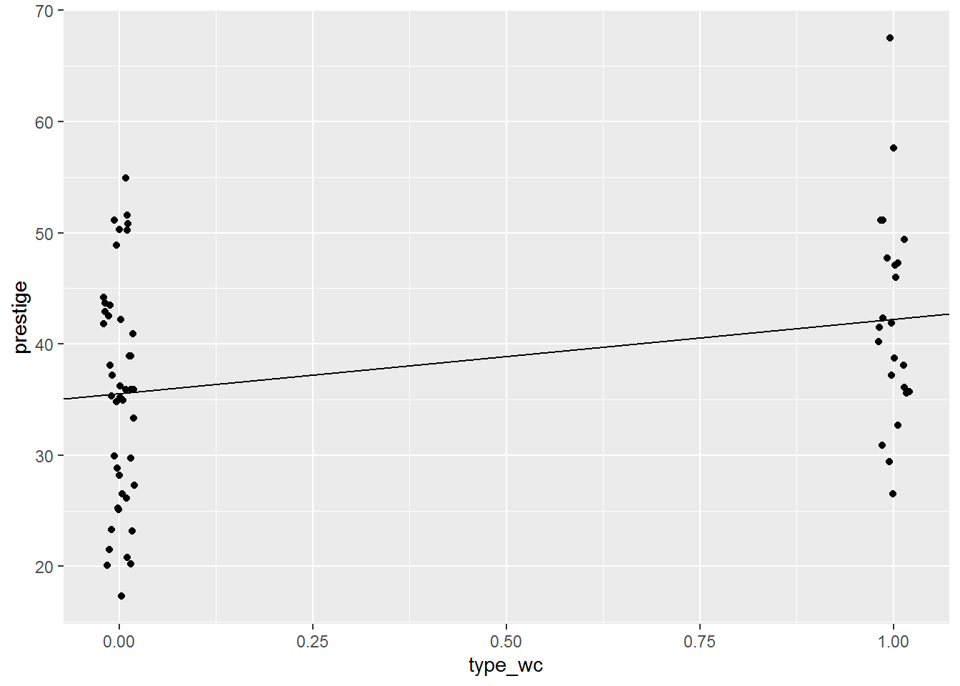

The values at the left hand side, above 0, are for blue collar occupations and at the right hand size, above 1, are for white collar occupations.

We asked lm to estimate an intercept ($\beta_0$) and slope for type_wc ($\beta_1$).

\[ \mathtt{prestige} = \beta_0 + \beta_1 \times \mathtt{type\_wc} \]

This is what it found:

\[ \mathtt{prestige} = 35.5 + 6.7 \times \mathtt{type\_wc} \]

Interpret the regression model as usual: for every unit increase in type_wc, prestige increases by 6.7. That’s the slope in the picture above.

But the type_wc variable only has two possible values, so this is the simplest example of “unit increase.” It can be 1, in which case we get the mean of white collar:

\[ \begin{array}{rcl} \mathtt{prestige} & = & 35.5 + 6.7 \times \mathtt{type\_wc}\\ & = & 35.5 + 6.7 \times 1 \\ & = & 35.5 + 6.7 \\ & = & 42.2 \end{array} \]

Alternatively, the predictor can be zero, in which case we get the mean of blue collar:

\[ \begin{array}{rcl} \mathtt{prestige} & = & 35.5 + 6.7 \times \mathtt{type\_wc}\\ & = & 35.5 + 6.7 \times 0 \\ & = & 35.5 + 0 \\ & = & 35.5 \end{array} \]

By the way, this is equivalent to a two-sample t-test assuming equal variance:

t.test(prestige ~ type, data = just_two, var.equal = TRUE)

## 
##  Two Sample t-test
## 
## data:  prestige by type
## t = -2.6487, df = 65, p-value = 0.01013
## alternative hypothesis: true difference in means is not equal to 0
## 95 percent confidence interval:
##  -11.780279  -1.652132
## sample estimates:
## mean in group bc mean in group wc 
##         35.52727         42.24348

7.6.3 Categorical predictors with 3 or more levels

In general, if a categorical variable has $n$ levels, then there will be $n-1$ binary predictors added to the regression model. One level must be chosen as the comparison level. Slopes for the predictors represent differences from that comparison level.

Here is a model, fitted using R’s automatic coding (and summarised with the aid of a pipe, just to add a little variation):

lm(prestige ~ type, data = dat_no_NAs) %>%
  summary()

## 
## Call:
## lm(formula = prestige ~ type, data = dat_no_NAs)
## 
## Residuals:
##      Min       1Q   Median       3Q      Max 
## -18.2273  -7.1773  -0.0854   6.1174  25.2565 
## 
## Coefficients:
##             Estimate Std. Error t value Pr(>|t|)    
## (Intercept)   35.527      1.432  24.810  < 2e-16 ***
## typeprof      32.321      2.227  14.511  < 2e-16 ***
## typewc         6.716      2.444   2.748  0.00718 ** 
## ---
## Signif. codes:  0 '***' 0.001 '**' 0.01 '*' 0.05 '.' 0.1 ' ' 1
## 
## Residual standard error: 9.499 on 95 degrees of freedom
## Multiple R-squared:  0.6976, Adjusted R-squared:  0.6913 
## F-statistic: 109.6 on 2 and 95 DF,  p-value: < 2.2e-16

Now let’s do the same again “by hand,” to show the coding:

dat_no_NAs$type_prof <- as.numeric(dat_no_NAs$type == "prof")
dat_no_NAs$type_wc   <- as.numeric(dat_no_NAs$type == "wc")

There are now two predictors: type_prof is 1 when the occupation type is prof and 0 otherwise; type_wc is 1 when the occupation type is wc and 0 otherwise. Whenever the occupation type is bc, both of these predictors are zero.

Have a look to see what this has done, comparing the type column with type_prof and type_wc:

dat_no_NAs

##                           occ prestige type type_prof type_wc
## 1          gov administrators     68.8 prof         1       0
## 2            general managers     69.1 prof         1       0
## 3                 accountants     63.4 prof         1       0
## 4         purchasing officers     56.8 prof         1       0
## 5                    chemists     73.5 prof         1       0
## 6                  physicists     77.6 prof         1       0
## 7                  biologists     72.6 prof         1       0
## 8                  architects     78.1 prof         1       0
## 9             civil engineers     73.1 prof         1       0
## 10           mining engineers     68.8 prof         1       0
## 11                  surveyors     62.0 prof         1       0
## 12                draughtsmen     60.0 prof         1       0
## 13        computer programers     53.8 prof         1       0
## 14                 economists     62.2 prof         1       0
## 15              psychologists     74.9 prof         1       0
## 16             social workers     55.1 prof         1       0
## 17                    lawyers     82.3 prof         1       0
## 18                 librarians     58.1 prof         1       0
## 19     vocational counsellors     58.3 prof         1       0
## 20                  ministers     72.8 prof         1       0
## 21        university teachers     84.6 prof         1       0
## 22    primary school teachers     59.6 prof         1       0
## 23  secondary school teachers     66.1 prof         1       0
## 24                 physicians     87.2 prof         1       0
## 25              veterinarians     66.7 prof         1       0
## 26   osteopaths chiropractors     68.4 prof         1       0
## 27                     nurses     64.7 prof         1       0
## 28              nursing aides     34.9   bc         0       0
## 29           physio therapsts     72.1 prof         1       0
## 30                pharmacists     69.3 prof         1       0
## 31        medical technicians     67.5   wc         0       1
## 32         commercial artists     57.2 prof         1       0
## 33        radio tv announcers     57.6   wc         0       1
## 35                secretaries     46.0   wc         0       1
## 36                    typists     41.9   wc         0       1
## 37                bookkeepers     49.4   wc         0       1
## 38           tellers cashiers     42.3   wc         0       1
## 39         computer operators     47.7   wc         0       1
## 40            shipping clerks     30.9   wc         0       1
## 41                file clerks     32.7   wc         0       1
## 42               receptionsts     38.7   wc         0       1
## 43              mail carriers     36.1   wc         0       1
## 44              postal clerks     37.2   wc         0       1
## 45        telephone operators     38.1   wc         0       1
## 46                 collectors     29.4   wc         0       1
## 47            claim adjustors     51.1   wc         0       1
## 48              travel clerks     35.7   wc         0       1
## 49              office clerks     35.6   wc         0       1
## 50          sales supervisors     41.5   wc         0       1
## 51      commercial travellers     40.2   wc         0       1
## 52               sales clerks     26.5   wc         0       1
## 54  service station attendant     23.3   bc         0       0
## 55           insurance agents     47.3   wc         0       1
## 56       real estate salesmen     47.1   wc         0       1
## 57                     buyers     51.1   wc         0       1
## 58               firefighters     43.5   bc         0       0
## 59                  policemen     51.6   bc         0       0
## 60                      cooks     29.7   bc         0       0
## 61                 bartenders     20.2   bc         0       0
## 62          funeral directors     54.9   bc         0       0
## 64                 launderers     20.8   bc         0       0
## 65                   janitors     17.3   bc         0       0
## 66         elevator operators     20.1   bc         0       0
## 68               farm workers     21.5   bc         0       0
## 69       rotary well drillers     35.3   bc         0       0
## 70                     bakers     38.9   bc         0       0
## 71             slaughterers 1     25.2   bc         0       0
## 72             slaughterers 2     34.8   bc         0       0
## 73                    canners     23.2   bc         0       0
## 74            textile weavers     33.3   bc         0       0
## 75          textile labourers     28.8   bc         0       0
## 76            tool die makers     42.5   bc         0       0
## 77                 machinists     44.2   bc         0       0
## 78        sheet metal workers     35.9   bc         0       0
## 79                    welders     41.8   bc         0       0
## 80               auto workers     35.9   bc         0       0
## 81           aircraft workers     43.7   bc         0       0
## 82         electronic workers     50.8   bc         0       0
## 83         radio tv repairmen     37.2   bc         0       0
## 84      sewing mach operators     28.2   bc         0       0
## 85             auto repairmen     38.1   bc         0       0
## 86         aircraft repairmen     50.3   bc         0       0
## 87         railway sectionmen     27.3   bc         0       0
## 88         electrical linemen     40.9   bc         0       0
## 89               electricians     50.2   bc         0       0
## 90       construction foremen     51.1   bc         0       0
## 91                 carpenters     38.9   bc         0       0
## 92                     masons     36.2   bc         0       0
## 93             house painters     29.9   bc         0       0
## 94                   plumbers     42.9   bc         0       0
## 95     construction labourers     26.5   bc         0       0
## 96                     pilots     66.1 prof         1       0
## 97            train engineers     48.9   bc         0       0
## 98                bus drivers     35.9   bc         0       0
## 99               taxi drivers     25.1   bc         0       0
## 100              longshoremen     26.1   bc         0       0
## 101               typesetters     42.2   bc         0       0
## 102               bookbinders     35.2   bc         0       0

If we fit a model with these two “hand coded” predictors, the results are identical to what R did automatically:

lm(prestige ~ type_prof + type_wc, data = dat_no_NAs) %>%
  summary()

## 
## Call:
## lm(formula = prestige ~ type_prof + type_wc, data = dat_no_NAs)
## 
## Residuals:
##      Min       1Q   Median       3Q      Max 
## -18.2273  -7.1773  -0.0854   6.1174  25.2565 
## 
## Coefficients:
##             Estimate Std. Error t value Pr(>|t|)    
## (Intercept)   35.527      1.432  24.810  < 2e-16 ***
## type_prof     32.321      2.227  14.511  < 2e-16 ***
## type_wc        6.716      2.444   2.748  0.00718 ** 
## ---
## Signif. codes:  0 '***' 0.001 '**' 0.01 '*' 0.05 '.' 0.1 ' ' 1
## 
## Residual standard error: 9.499 on 95 degrees of freedom
## Multiple R-squared:  0.6976, Adjusted R-squared:  0.6913 
## F-statistic: 109.6 on 2 and 95 DF,  p-value: < 2.2e-16

Now the formula is:

\[ \begin{array}{rcl} \mathtt{prestige} & = & 35.5 + 32.3 \times \mathtt{type\_prof} + 6.7 \times \mathtt{type\_wc} \end{array} \]

There are three possibilities:

type_prof and type_wc are both zero, so the model computes the mean prestige for blue collar workers.

\[ \begin{array}{rcl} \mathtt{prestige} & = & 35.5 + 32.3 \times 0 + 6.7 \times 0\\ & = & 35.5 \end{array} \]

type_prof is 1 and type_wc is 0, so the model computes the mean prestige for professionals.

\[ \begin{array}{rcl} \mathtt{prestige} & = & 35.5 + 32.3 \times 1 + 6.7 \times 0\\ & = & 35.5 + 32.3\\ & = & 67.8 \end{array} \]

type_prof is 0 and type_wc is 1, so the model computes the mean prestige for white collar workers.

\[ \begin{array}{rcl} \mathtt{prestige} & = & 35.5 + 32.3 \times 0 + 6.7 \times 1\\ & = & 35.5 + 6.7\\ & = & 42.2 \end{array} \]

7.7 Interpreting the coefficients

Here’s the model again:

lm(prestige ~ type, data = dat_no_NAs) %>%
  summary()

## 
## Call:
## lm(formula = prestige ~ type, data = dat_no_NAs)
## 
## Residuals:
##      Min       1Q   Median       3Q      Max 
## -18.2273  -7.1773  -0.0854   6.1174  25.2565 
## 
## Coefficients:
##             Estimate Std. Error t value Pr(>|t|)    
## (Intercept)   35.527      1.432  24.810  < 2e-16 ***
## typeprof      32.321      2.227  14.511  < 2e-16 ***
## typewc         6.716      2.444   2.748  0.00718 ** 
## ---
## Signif. codes:  0 '***' 0.001 '**' 0.01 '*' 0.05 '.' 0.1 ' ' 1
## 
## Residual standard error: 9.499 on 95 degrees of freedom
## Multiple R-squared:  0.6976, Adjusted R-squared:  0.6913 
## F-statistic: 109.6 on 2 and 95 DF,  p-value: < 2.2e-16

From this we can see that the prestige for professionals is 32.3 points more than for blue collar workers ($t = 14.5$, $p < .001$) and prestige for white collar workers is 6.7 points more than for blue collar ($t = 2.7$, $p = .007$); both differences are statistically significant.

We have a variable with three levels and this has ended up the regression model as two predictors, (1) typewc and (2) typeprof, the slopes of which represent the difference between (1) wc and bc and (2) prof and bc, respectively.

But this does not currently show us all combinations. What is the difference between wc and prof?

Here is relevel to the rescue. It relevels a factor so that whichever level you name comes first. You can add the command directly to a model specification like this:

lm(prestige ~ relevel(type, "prof"), data = dat_no_NAs) %>%
  summary()

## 
## Call:
## lm(formula = prestige ~ relevel(type, "prof"), data = dat_no_NAs)
## 
## Residuals:
##      Min       1Q   Median       3Q      Max 
## -18.2273  -7.1773  -0.0854   6.1174  25.2565 
## 
## Coefficients:
##                         Estimate Std. Error t value Pr(>|t|)    
## (Intercept)               67.848      1.706  39.770  < 2e-16 ***
## relevel(type, "prof")bc  -32.321      2.227 -14.511  < 2e-16 ***
## relevel(type, "prof")wc  -25.605      2.614  -9.795 4.53e-16 ***
## ---
## Signif. codes:  0 '***' 0.001 '**' 0.01 '*' 0.05 '.' 0.1 ' ' 1
## 
## Residual standard error: 9.499 on 95 degrees of freedom
## Multiple R-squared:  0.6976, Adjusted R-squared:  0.6913 
## F-statistic: 109.6 on 2 and 95 DF,  p-value: < 2.2e-16

Or, do it a longer but clearer way, e.g.,

dat_no_NAs$type_vs_prof <- relevel(dat_no_NAs$type, "prof")
myMod <- lm(prestige ~ type_vs_prof, data = dat_no_NAs)
summary(myMod)

## 
## Call:
## lm(formula = prestige ~ type_vs_prof, data = dat_no_NAs)
## 
## Residuals:
##      Min       1Q   Median       3Q      Max 
## -18.2273  -7.1773  -0.0854   6.1174  25.2565 
## 
## Coefficients:
##                Estimate Std. Error t value Pr(>|t|)    
## (Intercept)      67.848      1.706  39.770  < 2e-16 ***
## type_vs_profbc  -32.321      2.227 -14.511  < 2e-16 ***
## type_vs_profwc  -25.605      2.614  -9.795 4.53e-16 ***
## ---
## Signif. codes:  0 '***' 0.001 '**' 0.01 '*' 0.05 '.' 0.1 ' ' 1
## 
## Residual standard error: 9.499 on 95 degrees of freedom
## Multiple R-squared:  0.6976, Adjusted R-squared:  0.6913 
## F-statistic: 109.6 on 2 and 95 DF,  p-value: < 2.2e-16

The advantage of this is that we can have a look at the levels and check that prof comes first:

levels(dat_no_NAs$type_vs_prof)

## [1] "prof" "bc"   "wc"

7.7.1 Activity

Interpret the coefficients in this myMod model.

7.7.2 Answer

Prestige for professionals is 32.3 points greater than for blue collar workers ($t = 14.5$, $p < .001$) and 25.6 points greater than for white collar workers ($t = 9.8$, $p < .001$).

7.8 Checking all combinations

It can quickly become a pain to use relevel like this and there are various alternatives.

At this point, I wish I hadn’t been so clever using a pipe and instead just saved the model. I shall do so now.

das_Model <- lm(prestige ~ type, data = dat_no_NAs)

We will use the emmeans package.

library(emmeans)

The main function therein is emmeans. Fox and Weisberg (2019, p. 203) comment that the formula argument is “idiosyncratic.” Anyway, here is how to use it:

emmeans(das_Model, pairwise ~ type)

## $emmeans
##  type emmean   SE df lower.CL upper.CL
##  bc     35.5 1.43 95     32.7     38.4
##  prof   67.8 1.71 95     64.5     71.2
##  wc     42.2 1.98 95     38.3     46.2
## 
## Confidence level used: 0.95 
## 
## $contrasts
##  contrast  estimate   SE df t.ratio p.value
##  bc - prof   -32.32 2.23 95 -14.511 <.0001 
##  bc - wc      -6.72 2.44 95  -2.748 0.0195 
##  prof - wc    25.60 2.61 95   9.795 <.0001 
## 
## P value adjustment: tukey method for comparing a family of 3 estimates

The first parameter is the name of the model, the second is a formula specifying which comparisons are required. The idiosyncracy in the model specification is that “pairwise” is not a variable in the data – it’s a type of comparison.

Compare and contrast with the results obtained by using relevel above.

The estimates are identical. One difference you will observe is that the p-values are adjusted for the number of comparisons. There has been an enormous quantity of ink spilled on the problem of multiple comparisons. You may recall a variety of corrections, often named after their creators, e.g., Bonferroni, Bonferroni-Holm (my favourite), and Šidák.

Here, the p-values are adjusted by “tukey method” which is Tukey’s Honest Significant Differences (HSD) adjustment. (Tukey is another statistician.)

7.9 The intercept is not always the mean of the comparison group

The intercept always works the same way: it is the mean of the outcome variable when the predictors are zero. In the examples we have looked at, this was the mean of the comparison group – whatever happened to be the first level of the factor.

Let’s try another model:

more_data <- dat %>%
  select(occ, prestige, type, income) %>%
  na.omit()
type_and_income <- lm(prestige ~ I(income/1000) + type, data = more_data)
summary(type_and_income)

## 
## Call:
## lm(formula = prestige ~ I(income/1000) + type, data = more_data)
## 
## Residuals:
##      Min       1Q   Median       3Q      Max 
## -20.2141  -6.7359  -0.1931   5.1725  25.0776 
## 
## Coefficients:
##                Estimate Std. Error t value Pr(>|t|)    
## (Intercept)     27.9971     1.8008  15.547  < 2e-16 ***
## I(income/1000)   1.4012     0.2434   5.757 1.07e-07 ***
## typeprof        25.0555     2.3020  10.884  < 2e-16 ***
## typewc           7.1672     2.1140   3.390  0.00102 ** 
## ---
## Signif. codes:  0 '***' 0.001 '**' 0.01 '*' 0.05 '.' 0.1 ' ' 1
## 
## Residual standard error: 8.21 on 94 degrees of freedom
## Multiple R-squared:  0.7765, Adjusted R-squared:  0.7693 
## F-statistic: 108.8 on 3 and 94 DF,  p-value: < 2.2e-16

Now the intercept is not the mean prestige for blue collar workers, but rather it is predicted mean prestige for blue collar workers when income is zero.

By the way, we can use emmeans again to compare occupation types, holding income constant:

emmeans(type_and_income, pairwise ~ type)

## $emmeans
##  type emmean   SE df lower.CL upper.CL
##  bc     37.7 1.30 94     35.1     40.3
##  prof   62.8 1.72 94     59.4     66.2
##  wc     44.9 1.77 94     41.4     48.4
## 
## Confidence level used: 0.95 
## 
## $contrasts
##  contrast  estimate   SE df t.ratio p.value
##  bc - prof   -25.06 2.30 94 -10.884 <.0001 
##  bc - wc      -7.17 2.11 94  -3.390 0.0029 
##  prof - wc    17.89 2.63 94   6.809 <.0001 
## 
## P value adjustment: tukey method for comparing a family of 3 estimates

7.10 Recap

Okay, we have covered rather a lot of ground there so let me summarise a swift method for testing whether a categorical predictor explains variance in some outcome. I’ll use an example where we also statistically adjust for another predictor (known as a covariate).

First, do whatever you need to do to obtain and tidy the data:

more_data <- dat %>%
  select(occ, prestige, type, income) %>%
  na.omit()

Fit the model of interest:

my_model <- lm(prestige ~ I(income/1000) + type, data = more_data)

Use Anova to see which predictors are statistically significant

Anova(my_model)

## Anova Table (Type II tests)
## 
## Response: prestige
##                Sum Sq Df F value    Pr(>F)    
## I(income/1000) 2234.5  1  33.147 1.068e-07 ***
## type           7988.5  2  59.251 < 2.2e-16 ***
## Residuals      6336.7 94                      
## ---
## Signif. codes:  0 '***' 0.001 '**' 0.01 '*' 0.05 '.' 0.1 ' ' 1

Look at a summary:

summary(my_model)

## 
## Call:
## lm(formula = prestige ~ I(income/1000) + type, data = more_data)
## 
## Residuals:
##      Min       1Q   Median       3Q      Max 
## -20.2141  -6.7359  -0.1931   5.1725  25.0776 
## 
## Coefficients:
##                Estimate Std. Error t value Pr(>|t|)    
## (Intercept)     27.9971     1.8008  15.547  < 2e-16 ***
## I(income/1000)   1.4012     0.2434   5.757 1.07e-07 ***
## typeprof        25.0555     2.3020  10.884  < 2e-16 ***
## typewc           7.1672     2.1140   3.390  0.00102 ** 
## ---
## Signif. codes:  0 '***' 0.001 '**' 0.01 '*' 0.05 '.' 0.1 ' ' 1
## 
## Residual standard error: 8.21 on 94 degrees of freedom
## Multiple R-squared:  0.7765, Adjusted R-squared:  0.7693 
## F-statistic: 108.8 on 3 and 94 DF,  p-value: < 2.2e-16

Use emmeans to check for any comparisons of interest which were not included in the way the factor was initially setup:

emmeans(my_model, pairwise ~ type)

## $emmeans
##  type emmean   SE df lower.CL upper.CL
##  bc     37.7 1.30 94     35.1     40.3
##  prof   62.8 1.72 94     59.4     66.2
##  wc     44.9 1.77 94     41.4     48.4
## 
## Confidence level used: 0.95 
## 
## $contrasts
##  contrast  estimate   SE df t.ratio p.value
##  bc - prof   -25.06 2.30 94 -10.884 <.0001 
##  bc - wc      -7.17 2.11 94  -3.390 0.0029 
##  prof - wc    17.89 2.63 94   6.809 <.0001 
## 
## P value adjustment: tukey method for comparing a family of 3 estimates

Don’t forget to check model diagnostics…

7.11 Challenge

7.11.1 Activity

Fit a regression model with income as the outcome variable and occupation type as a predictor. Does type explain variance in outcome?
Is there a statistically significant difference between blue collar and white collar salaries?
Is there a statistically significant difference between white collar and professional salaries?
Are the residuals normally distributed?
Try logging income to see what impact it has on the residual distribution
Now compare all differences between groups

7.11.2 Answers

a. Fit a regression model with income as the outcome variable and occupation type as a predictor. Does type explain variance in outcome?

income_mod <- lm(income ~ type, data = dat)
Anova(income_mod)

## Anova Table (Type II tests)
## 
## Response: income
##               Sum Sq Df F value    Pr(>F)    
## type       595956156  2  24.872 2.057e-09 ***
## Residuals 1138123006 95                      
## ---
## Signif. codes:  0 '***' 0.001 '**' 0.01 '*' 0.05 '.' 0.1 ' ' 1

Yes: $F(2,95) = 24.87$, $p < .001$

b. Is there a statistically significant difference between blue collar and white collar salaries?

First, let’s have a look at the means, to help aid interpretation:

dat %>%
  group_by(type) %>%
  summarise(mean_income = mean(income))

## # A tibble: 4 x 2
##   type  mean_income
##   <fct>       <dbl>
## 1 bc          5374.
## 2 prof       10559.
## 3 wc          5052.
## 4 <NA>        3344.

The means for blue collar and white collar look very similar, about $300 difference. Let’s test that difference:

summary(income_mod)

## 
## Call:
## lm(formula = income ~ type, data = dat)
## 
## Residuals:
##     Min      1Q  Median      3Q     Max 
## -5945.5 -2003.3  -466.2  1536.9 15319.5 
## 
## Coefficients:
##             Estimate Std. Error t value Pr(>|t|)    
## (Intercept)   5374.1      521.8  10.299  < 2e-16 ***
## typeprof      5185.3      811.6   6.389 6.16e-09 ***
## typewc        -321.8      890.6  -0.361    0.719    
## ---
## Signif. codes:  0 '***' 0.001 '**' 0.01 '*' 0.05 '.' 0.1 ' ' 1
## 
## Residual standard error: 3461 on 95 degrees of freedom
##   (4 observations deleted due to missingness)
## Multiple R-squared:  0.3437, Adjusted R-squared:  0.3299 
## F-statistic: 24.87 on 2 and 95 DF,  p-value: 2.057e-09

There is no statistically significant difference, $t = 0.361$, $p = .71$.

c. Is there a statistically significant difference between white collar and professional salaries?

We can refit the model using relevel like so:

income_mod_wc <- lm(income ~ relevel(type, "wc"), data = dat)
summary(income_mod_wc)

## 
## Call:
## lm(formula = income ~ relevel(type, "wc"), data = dat)
## 
## Residuals:
##     Min      1Q  Median      3Q     Max 
## -5945.5 -2003.3  -466.2  1536.9 15319.5 
## 
## Coefficients:
##                         Estimate Std. Error t value Pr(>|t|)    
## (Intercept)               5052.3      721.7   7.000  3.6e-10 ***
## relevel(type, "wc")bc      321.8      890.6   0.361    0.719    
## relevel(type, "wc")prof   5507.1      952.5   5.782  9.4e-08 ***
## ---
## Signif. codes:  0 '***' 0.001 '**' 0.01 '*' 0.05 '.' 0.1 ' ' 1
## 
## Residual standard error: 3461 on 95 degrees of freedom
##   (4 observations deleted due to missingness)
## Multiple R-squared:  0.3437, Adjusted R-squared:  0.3299 
## F-statistic: 24.87 on 2 and 95 DF,  p-value: 2.057e-09

Yes, professional salaries are a mean $5507 more than white collar salaries ($t = 5.78$, $p < .001$).

d. Are the residuals normally distributed?

The order of levels does not affect the residuals, so either model would do:

qqPlot(resid(income_mod_wc))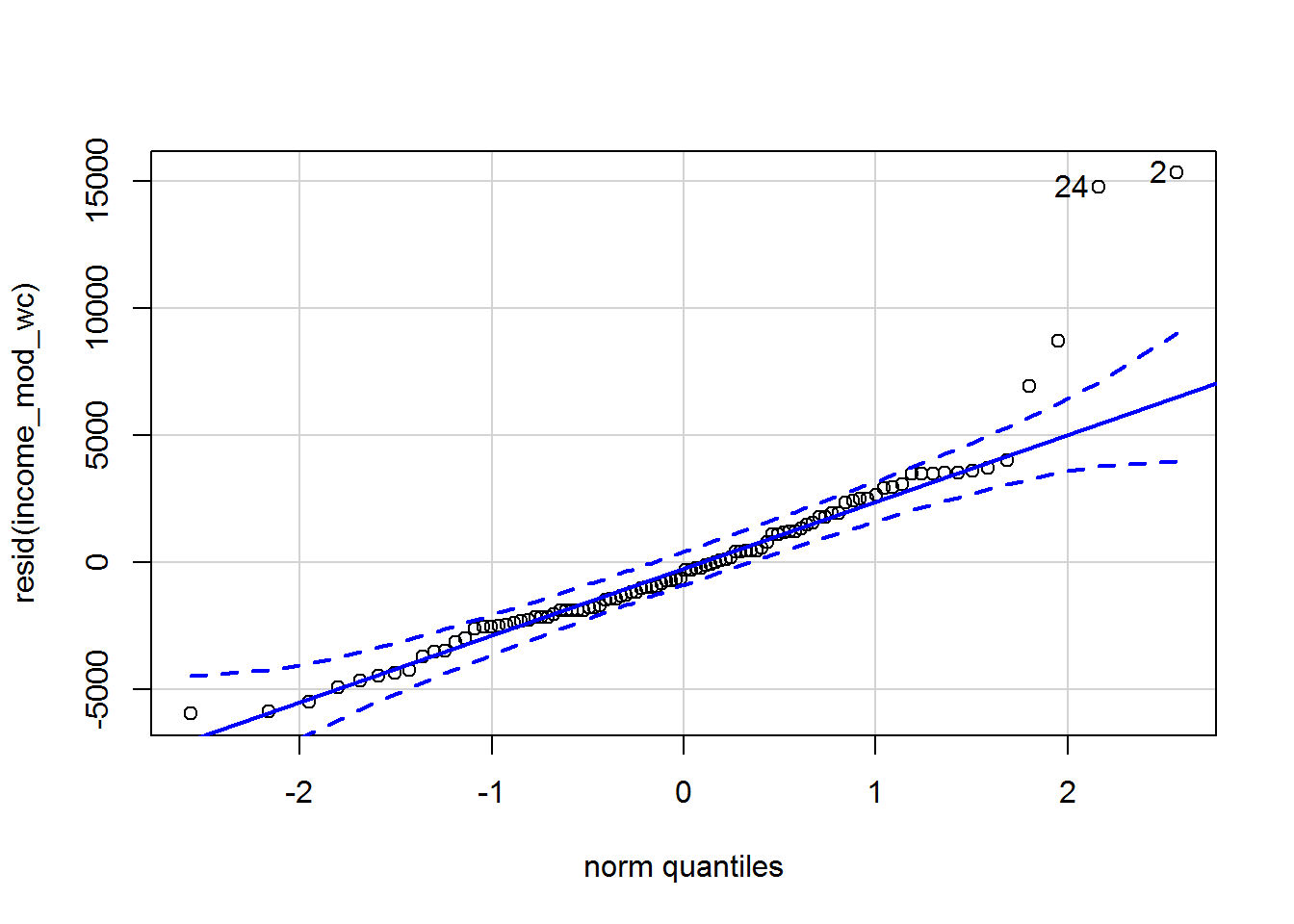

## [1]  2 24

Hmmmm something fishy for residuals above 5000. Let’s look at the histogram in case it is more obvious:

hist(resid(income_mod_wc))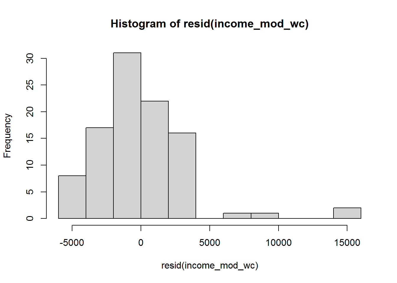

Looks like they are not normally distributed, though maybe driven by outliers?

e. Try logging income to see what impact it has on the residual distribution

dat$log_income <- log(dat$income)
log_income_mod <- lm(log_income ~ type, data = dat)

Now the residuals look much better:

qqPlot(resid(log_income_mod))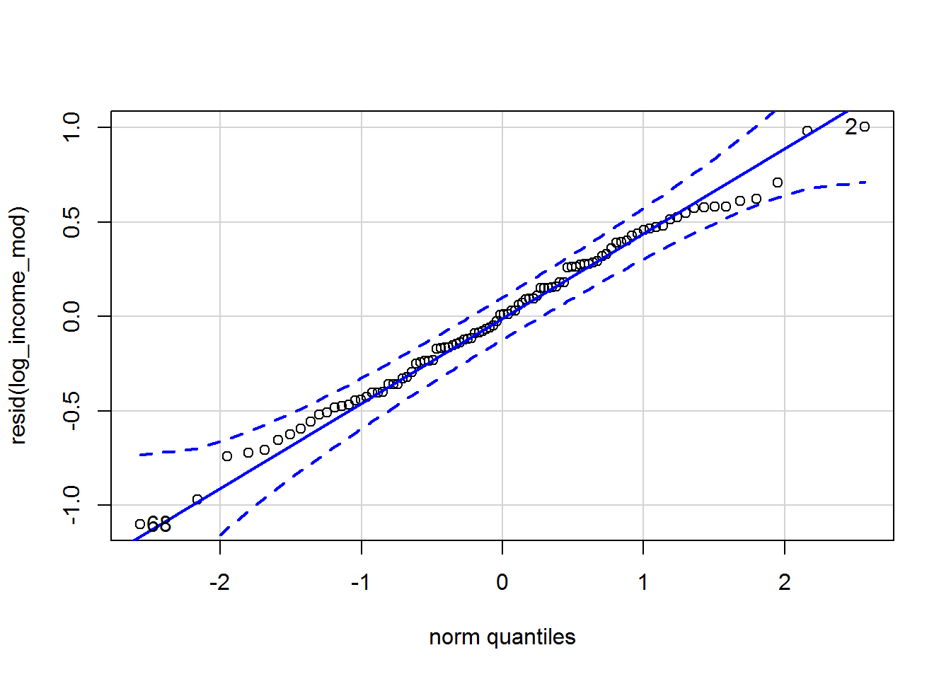

## 68  2 
## 64  2

f. Now compare all differences between groups

Let’s use emmeans:

emmeans(log_income_mod, pairwise ~ type)

## $emmeans
##  type emmean     SE df lower.CL upper.CL
##  bc     8.51 0.0638 95     8.39     8.64
##  prof   9.16 0.0760 95     9.01     9.31
##  wc     8.46 0.0882 95     8.28     8.63
## 
## Confidence level used: 0.95 
## 
## $contrasts
##  contrast  estimate     SE df t.ratio p.value
##  bc - prof  -0.6452 0.0992 95 -6.507  <.0001 
##  bc - wc     0.0562 0.1088 95  0.516  0.8636 
##  prof - wc   0.7014 0.1164 95  6.027  <.0001 
## 
## P value adjustment: tukey method for comparing a family of 3 estimates

Note that the estimates are on the log scale, e.g., the difference between professional and white collar salaries is 0.7 on the logged $1000s scale.

7.12 Brief introduction to interactions

Fox and Weisberg (2019, pp. 207-224) say lots about interactions. In this tutorial I just want to mention briefly what they are and how to ask R to model them.

7.12.1 What is an interaction?

An interaction between two variables simply means that the relationship between the outcome and one of the variables is changed (or “moderated”) by the other variable. For example, we found that occupation type explains variation in prestige. It is possible that the magnitude of differences between occupation types depend on mean income.

Interactions can also be used to test for intersectional effects. Discrimination may, for instance, depend on sexism and racism – both operate independently. However, additionally the differences between men and women on some variable like salary might also depend on ethnicity and/or on whether you are cisgender or transgender.

Arithmetically, an interaction between two variables, A and B is represented as a new variable which is A and B multiplied together. R does the coding for us.

7.12.2 How to test for interactions in R

This shows how to test for an interaction between income and occupation type.

Let’s select some data again:

dat_for_int <- dat %>%
  select(occ, prestige, type, income) %>%
  na.omit()

First, predict prestige from income (in thousands) and occupation type. This model has the so-called “main effects,” i.e., without any interaction.

dat$income_1000s <- dat$income/1000
main_effect_mod <- lm(prestige ~ income_1000s + type, data = dat)
summary(main_effect_mod)

## 
## Call:
## lm(formula = prestige ~ income_1000s + type, data = dat)
## 
## Residuals:
##      Min       1Q   Median       3Q      Max 
## -20.2141  -6.7359  -0.1931   5.1725  25.0776 
## 
## Coefficients:
##              Estimate Std. Error t value Pr(>|t|)    
## (Intercept)   27.9971     1.8008  15.547  < 2e-16 ***
## income_1000s   1.4012     0.2434   5.757 1.07e-07 ***
## typeprof      25.0555     2.3020  10.884  < 2e-16 ***
## typewc         7.1672     2.1140   3.390  0.00102 ** 
## ---
## Signif. codes:  0 '***' 0.001 '**' 0.01 '*' 0.05 '.' 0.1 ' ' 1
## 
## Residual standard error: 8.21 on 94 degrees of freedom
##   (4 observations deleted due to missingness)
## Multiple R-squared:  0.7765, Adjusted R-squared:  0.7693 
## F-statistic: 108.8 on 3 and 94 DF,  p-value: < 2.2e-16

We can then use Anova as before:

Anova(main_effect_mod)

## Anova Table (Type II tests)
## 
## Response: prestige
##              Sum Sq Df F value    Pr(>F)    
## income_1000s 2234.5  1  33.147 1.068e-07 ***
## type         7988.5  2  59.251 < 2.2e-16 ***
## Residuals    6336.7 94                      
## ---
## Signif. codes:  0 '***' 0.001 '**' 0.01 '*' 0.05 '.' 0.1 ' ' 1

There are effects for both income ($F(1,94) = 33.1$, $p < .001$) and occupation type ($F(2,94) = 59.3$, $p < .001$).

Now, do differences between occupation types depend on income?

We can check as follows:

interaction_mod <- lm(prestige ~ income_1000s + type +
                        income_1000s:type,
                      data = dat)
anova(main_effect_mod, interaction_mod)

## Analysis of Variance Table
## 
## Model 1: prestige ~ income_1000s + type
## Model 2: prestige ~ income_1000s + type + income_1000s:type
##   Res.Df    RSS Df Sum of Sq      F    Pr(>F)    
## 1     94 6336.7                                  
## 2     92 4859.2  2    1477.5 13.987 4.969e-06 ***
## ---
## Signif. codes:  0 '***' 0.001 '**' 0.01 '*' 0.05 '.' 0.1 ' ' 1

And the answer is, yes; $F(2,92) = 14.0$, $p < .001$.

It is also possible to check both main effects (without interactions) and the interaction effect in one go:

Anova(interaction_mod)

## Anova Table (Type II tests)
## 
## Response: prestige
##                   Sum Sq Df F value    Pr(>F)    
## income_1000s      2234.5  1  42.306 3.999e-09 ***
## type              7988.5  2  75.623 < 2.2e-16 ***
## income_1000s:type 1477.5  2  13.987 4.969e-06 ***
## Residuals         4859.2 92                      
## ---
## Signif. codes:  0 '***' 0.001 '**' 0.01 '*' 0.05 '.' 0.1 ' ' 1

The line beginning income_1000s:type shows the test of the interaction. To find out more about the Anova command and the Type II sum of squares it calculates by default, see Fox and Weisberg (2019, p. 262-264).

7.12.3 Understanding interactions

The most challenging aspect of interactions is that one can rapidly end up with enormously complex models which are difficult to interpret, even if everything is “statistically significant.” The secret to making sense of them is to plot model predictions. We will explore the ggeffects package – one easy way to do this – in more depth when examining logistic regression, but here is a preview of how it helps:

library(ggeffects)
ggpredict(interaction_mod, terms = c("income_1000s", "type")) %>%
  plot(add.data = TRUE, ci = FALSE)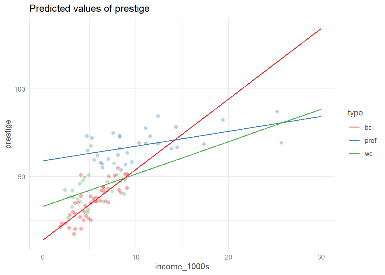

Hopefully this graph illustrates what it means that the relationship between income and prestige depends on occupation type – the slopes are different for each type.

We can also see what the model predictions look like without the interaction term:

library(ggeffects)
ggpredict(main_effect_mod, terms = c("income_1000s", "type")) %>%
  plot(add.data = TRUE, ci = FALSE)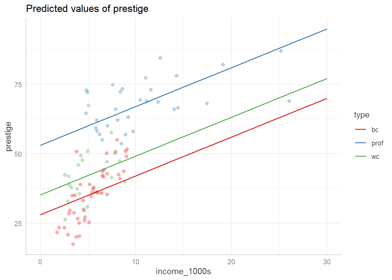

7.12.4 Further reading

You might be interested in Johnson-Neyman intervals. See the interactions package.