Chapter 9 Complex surveys
By the end of this chapter you will know how to:
- Setup a survey object using complex survey information such as sampling weight and stratification variables.
- Use a tidyverse-esq approach for descriptive statistics.
- Fit a GLM (logistic).
We will use the survey package and a tidyverse-style wrapper called srvyr.
library(survey)
library(srvyr)
9.1 Readings
These are handy:
srvyrcompared to thesurveypackage explains a way to use survey data in the tidyverse.- Fox and Weisberg’s online appendix, Fitting Regression Models to Data From Complex Surveys.
- The main reference for the models implemented by
surveyis the (expensive) book by Lumley (2010). - UCLA has extensive notes from a 2020 seminar on survey analysis.
- Analyzing international survey data with the pewmethods R package, by Kat Devlin, explains an alternative way to use weights for descriptive stats.
9.2 The dataset
This chapter’s dataset is drawn from the 2011 Canadian National Election Study – taken from the carData package and described by the Fox and Weisberg appendix cited above. Download it here.
There are 2231 observations on the following 9 variables:
| Variable name | Description |
|---|---|
| id | Household ID number. |
| province | a factor with (alphabetical) levels AB, BC, MB, NB, NL, NS, ON, PE, QC, SK; the sample was stratified by province. |
| population | population of the respondent’s province, number over age 17. |
| weight | weight sample to size of population, taking into account unequal sampling probabilities by province and household size. |
| gender | a factor with levels Female, Male. |
| abortion | attitude toward abortion, a factor with levels No, Yes; answer to the question “Should abortion be banned?” |
| importance | importance of religion, a factor with (alphabetical) levels not, notvery, somewhat, very; answer to the question, “In your life, would you say that religion is very important, somewhat important, not very important, or not important at all?” |
| education | a factor with (alphabetical) levels bachelors (Bachelors degree), college (community college or technical school), higher (graduate degree), HS (high-school graduate), lessHS (less than high-school graduate), somePS (some post-secondary). |
| urban | place of residence, a factor with levels rural, urban. |
Read in the data.
ces <- read.csv("ces11.csv", stringsAsFactors = TRUE)I’m setting stringsAsFactors to TRUE so that the variables which are obviously factors are setup accordingly (R used to this by default; sometimes it had irritating side-effects).
9.3 The components of a survey design
The key parts of the dataset which describe the survey design are as follows:
ces %>% select(id, province, population, weight) %>%
  head(6)
## id province population weight
## 1 2851 BC 3267345 4287.85
## 2 521 QC 5996930 9230.78
## 3 2118 QC 5996930 6153.85
## 4 1815 NL 406455 3430.00
## 5 1799 ON 9439960 8977.61
## 6 1103 ON 9439960 8977.61idis a unique identifier for each individual, which is particularly important when there is more than one data point per person, e.g., for multilevel modelling (not in this dataset).provincethe data were stratified by province – random sampling by landline numbers was done within province.populationprovides the population by province.weightis the sampling weight, in this dataset calculated based on differences in province population, the study sample size therein, and household size.
Here is how to setup a survey object using srvyr:
ces_s <- ces %>%
  as_survey(ids = id,
            strata = province,
            fpc = population,
            weights = weight)
9.4 Describing the data
We will sometimes want to compare weighted and unweighted analyses. Here is a warmup activity to show how using the tidyverse.
9.4.1 Activity
- use the
cesdata frame andtidyverseto calculate the number of people who think abortion should be banned - do the same again, but this time use the
ces_ssurvey object created above – what do you notice? - compare the proportions saying
yesby group
Hint: you will want to use group_by.
Another hint: to count, use the function n. The version for survey objects is called survey_total.
9.4.2 Answer
a. use the ces data frame and tidyverse to calculate the number of people who think abortion should be banned
ces %>%
  group_by(abortion) %>%
  summarise(n = n())
## `summarise()` ungrouping output (override with `.groups` argument)## # A tibble: 2 x 2
## abortion n
## <fct> <int>
## 1 No 1818
## 2 Yes 413b. do the same again, but this time use the ces_s survey object created above – what do you notice?
ces_s %>%
  group_by(abortion) %>%
  summarise(n = survey_total())
## # A tibble: 2 x 3
## abortion n n_se
## <fct> <dbl> <dbl>
## 1 No 13059520. 196984.
## 2 Yes 2964018. 162360.The counts are much bigger than the number of rows in the dataset due to the sampling weights.
c. compare the proportions saying yes by group
One way to do this is by copy and paste!
Unweighted:
prop_unweighted <- 413 / (413 + 1818)
prop_unweighted
## [1] 0.1851188Weighted:
prop_weighted <- 2964018 / (2964018 +   13059520)
prop_weighted
## [1] 0.184979The unweighted proportion of “yes” is only a little different in this case: 0.1851188 (unweighted) v 0.184979 (weighted).
Here’s how to answer the questions in one go:
ces_s %>%
  group_by(abortion) %>%
  summarise(n_raw = unweighted(n()),
            n_weighted = survey_total()) %>%
  mutate(prop_raw = n_raw / sum(n_raw),
         prop_weighted = n_weighted / sum(n_weighted)) %>%
  select(-n_weighted_se)
## # A tibble: 2 x 5
## abortion n_raw n_weighted prop_raw prop_weighted
## <fct> <int> <dbl> <dbl> <dbl>
## 1 No 1818 13059520. 0.815 0.815
## 2 Yes 413 2964018. 0.185 0.1859.5 Fitting a GLM
The survey package makes this very easy. There is a command called svyglm which is identical to glm except it has parameter called design instead of data.
See ?svyglm
9.5.1 Activity
mutatethe survey object to add a binary variable calledagainstAbortionwhich is 1 if the participant is against abortion and 0 if not.- fit an intercept-only logistic regression model without using weights (you can use
as_tibbleto get the “raw” data frame hidden within the survey object). - Do the same again, this time using the survey structure.
- compare the predicted proportions with the “raw” proportions we calculated earlier
9.5.2 Answer
a. mutate the survey object to add a binary variable called againstAbortion which is 1 if the participant is against abortion and 0 if not.
ces_s <- ces_s %>%
  mutate(againstAbortion = as.numeric(ces$abortion == "Yes"))
b. fit an intercept-only logistic regression model without using weights (you can use as_tibble to get the “raw” data frame hidden within the survey object).
m0 <- glm(againstAbortion ~ 1,
          data = as_tibble(ces_s),
          family = binomial)
summary(m0)
##
## Call:
## glm(formula = againstAbortion ~ 1, family = binomial, data = as_tibble(ces_s))
##
## Deviance Residuals:
## Min 1Q Median 3Q Max
## -0.6399 -0.6399 -0.6399 -0.6399 1.8367
##
## Coefficients:
## Estimate Std. Error z value Pr(>|z|)
## (Intercept) -1.48204 0.05451 -27.19 <2e-16 ***
## ---
## Signif. codes: 0 '***' 0.001 '**' 0.01 '*' 0.05 '.' 0.1 ' ' 1
##
## (Dispersion parameter for binomial family taken to be 1)
##
## Null deviance: 2137.6 on 2230 degrees of freedom
## Residual deviance: 2137.6 on 2230 degrees of freedom
## AIC: 2139.6
##
## Number of Fisher Scoring iterations: 4c. Do the same again, this time using the survey structure.
sm0 <- svyglm(againstAbortion ~ 1, design = ces_s,
              family = binomial)
## Warning in eval(family$initialize): non-integer #successes in a binomial glm!summary(sm0)##
## Call:
## svyglm(formula = againstAbortion ~ 1, design = ces_s, family = binomial)
##
## Survey design:
## Called via srvyr
##
## Coefficients:
## Estimate Std. Error t value Pr(>|t|)
## (Intercept) -1.48297 0.06534 -22.7 <2e-16 ***
## ---
## Signif. codes: 0 '***' 0.001 '**' 0.01 '*' 0.05 '.' 0.1 ' ' 1
##
## (Dispersion parameter for binomial family taken to be 1.000448)
##
## Number of Fisher Scoring iterations: 4d. compare the predicted proportions with the “raw” proportions we calculated earlier
This undoes the log-odds (logit) transform:
exp(coef(m0)) / (1+exp(coef(m0)))## (Intercept)
## 0.1851188exp(coef(sm0)) / (1+exp(coef(sm0)))## (Intercept)
## 0.184979The answer is the same as for the simple unweighted and weighted proportions, respectively.
9.6 Slopes
Now, having completed the traditional step of fitting an intercept-only model, we can give the slopes a go.
The Anova command in the car package works for svyglm models as before.
9.6.1 Activity
Regress againstAbortion on importance, education, and gender, and interpret what you find.
9.6.2 Answer
sm1 <- svyglm(againstAbortion ~ importance + education + gender,
              design = ces_s,
              family = binomial)
## Warning in eval(family$initialize): non-integer #successes in a binomial glm!summary(sm1)##
## Call:
## svyglm(formula = againstAbortion ~ importance + education + gender,
## design = ces_s, family = binomial)
##
## Survey design:
## Called via srvyr
##
## Coefficients:
## Estimate Std. Error t value Pr(>|t|)
## (Intercept) -3.8204 0.2962 -12.897 < 2e-16 ***
## importancenotvery 0.4606 0.3481 1.323 0.1858
## importancesomewhat 1.3287 0.2715 4.894 1.06e-06 ***
## importancevery 3.1405 0.2619 11.993 < 2e-16 ***
## educationcollege 0.4452 0.2278 1.954 0.0508 .
## educationhigher 0.3301 0.3046 1.084 0.2786
## educationHS 0.5692 0.2269 2.508 0.0122 *
## educationlessHS 1.0307 0.2468 4.177 3.07e-05 ***
## educationsomePS 0.1439 0.2806 0.513 0.6081
## genderMale 0.3299 0.1482 2.225 0.0261 *
## ---
## Signif. codes: 0 '***' 0.001 '**' 0.01 '*' 0.05 '.' 0.1 ' ' 1
##
## (Dispersion parameter for binomial family taken to be 0.973961)
##
## Number of Fisher Scoring iterations: 5To interpret those categorical predictors, it will help to check what the levels are:
levels(ces$importance)## [1] "not" "notvery" "somewhat" "very"So “not” is the comparison level.
levels(ces$education) ## [1] "bachelors" "college" "higher" "HS" "lessHS" "somePS"“bachelors” is the comparison level.
Gender is just a binary.
Example interpretations:
Men were more likely to be against abortion (log-odds 0.33 more)
People for whom religion was very important were more likely than those who said “not important at all” to be against abortion (log-odds 3.14)
You could get the odds ratios like so:
exp(coef(sm1)) %>% round(2)## (Intercept) importancenotvery importancesomewhat importancevery
## 0.02 1.59 3.78 23.12
## educationcollege educationhigher educationHS educationlessHS
## 1.56 1.39 1.77 2.80
## educationsomePS genderMale
## 1.15 1.39So the odds ratio of “very” versus “not” important is 23.1.
The ggeffects package also works with survey models (hurrah):
library(ggeffects)
ggeffect(sm1, terms = c("education", "importance"))  %>%
  plot() +
  ylim(0,1)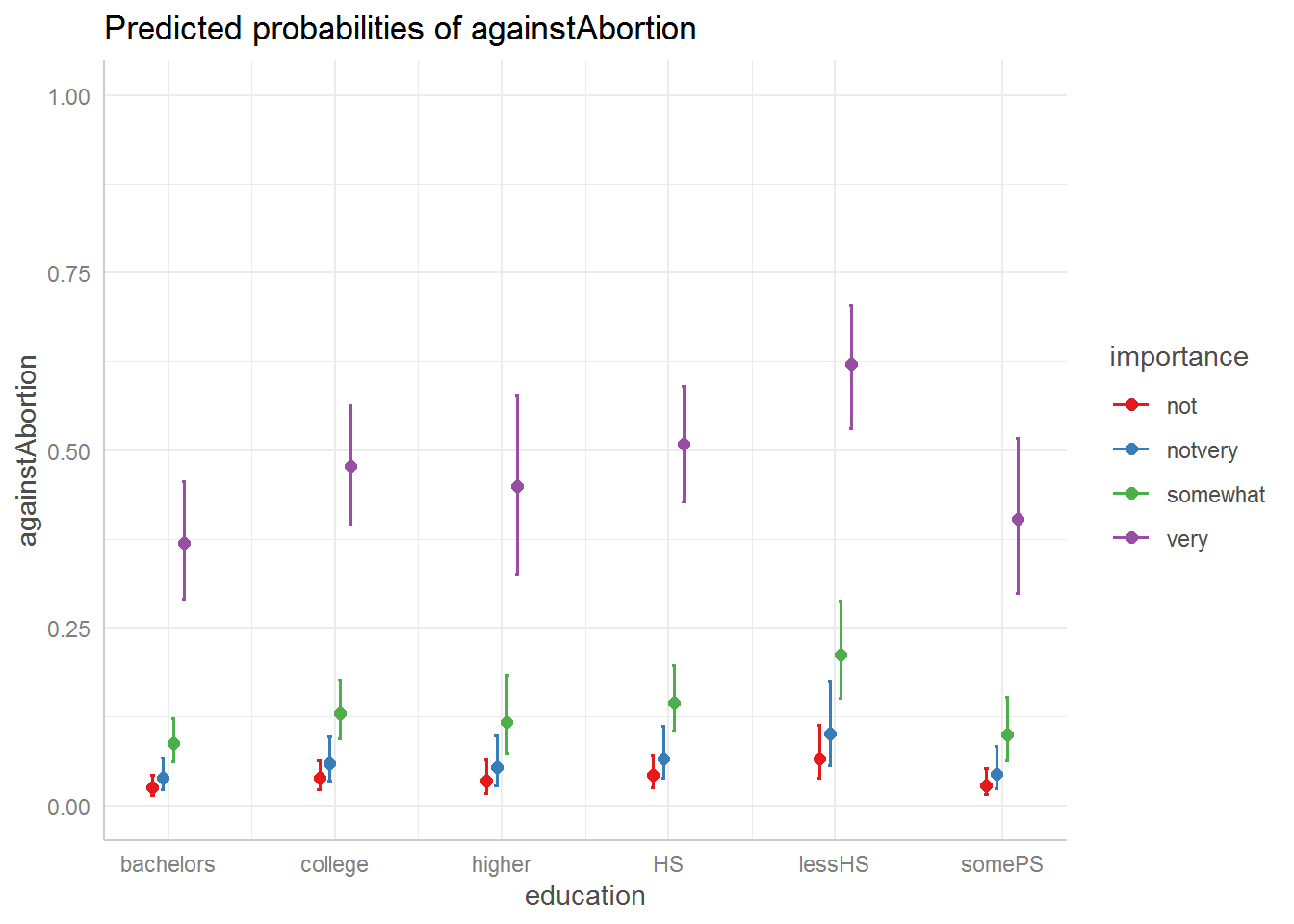
9.7 Diagnostics
Many of the diagnostic checks we previously encountered work here too.
Here are the VIFs:
vif(sm1)## GVIF Df GVIF^(1/(2*Df))
## importance 1.052799 3 1.008612
## education 1.066741 5 1.006482
## gender 1.039299 1 1.019460My favorite, the DFBETA plots:
dfbetaPlots(sm1)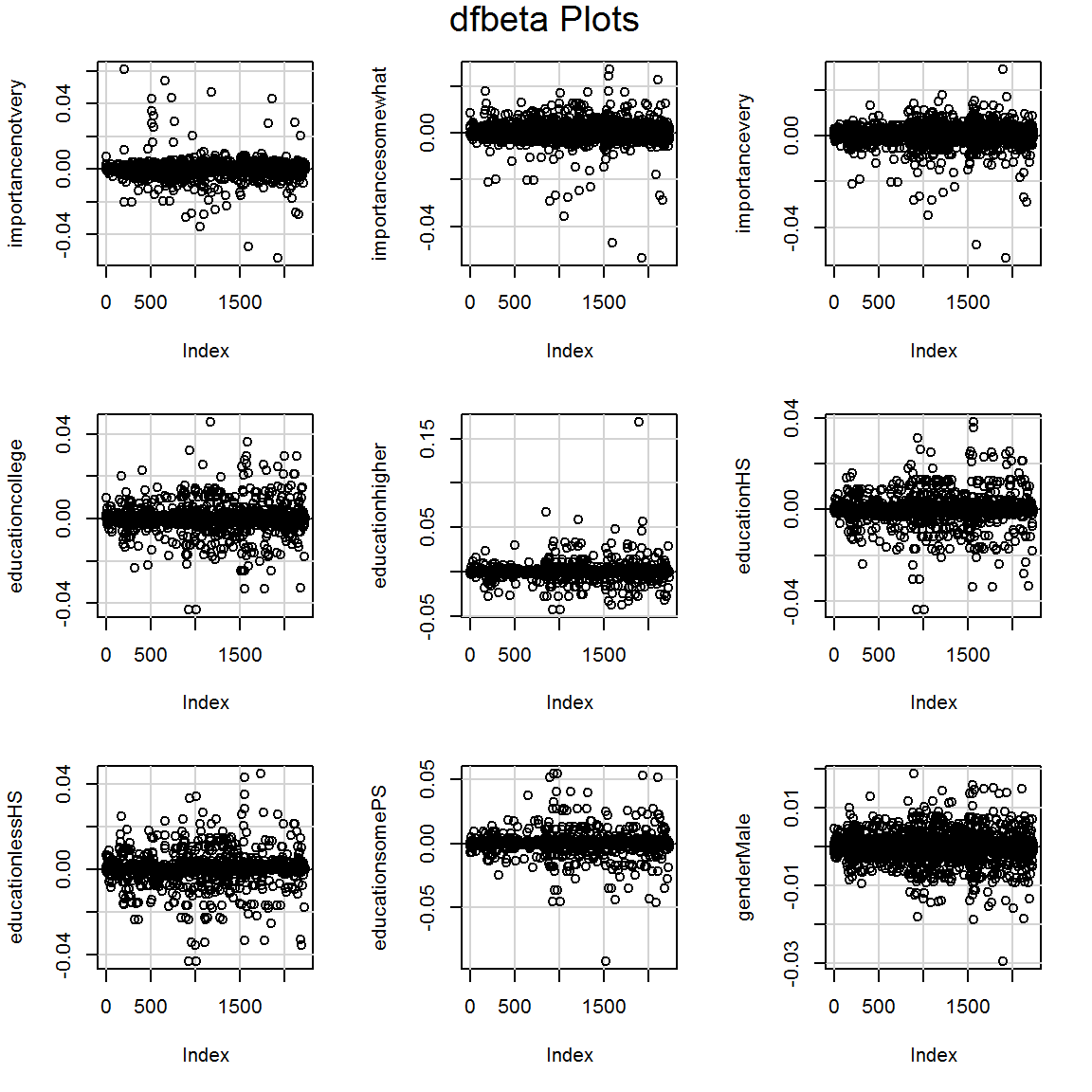
Try also:
influence.measures(sm1)9.8 Another worked example: the European Social Survey
NatCen recently published analyses of views on fairness and justice in Britain (Curtice, Hudson, & Montagu, 2020), using data from the ninth wave of the 2019 European Social Survey (European Social Survey Round 9 Data, 2018).
Let’s see if we can replicate the results.
Firstly, you will have to download the data from the ESS website. Go for the SPSS version. (You will have to register but it is a very quick process.) It will arrive as a zip file (ESS9e02.spss.zip). Simply extract the SPSS file therein (ESS9e02.sav) and move it to the same folder as your Markdown file.
library(haven)
ess9 <- read_sav("ESS9e02.sav")
Try having a look:
View(ess9)Okay, if that has worked then the next problem is finding the variables we want to analyse!
The report opens with a spotlight figure:
Only 20% of the British public think that differences in wealth in Britain are fair, whilst a majority (59%) think that wealth differences in Britain are unfairly large and a further 16% think that differences in wealth are unfairly small.
The question asked was:
In your opinion, are differences in wealth in Britain unfairly small, fair, or unfairly large?
It’s a good exercise to spend some time wading through the documentation on the ESS website to find the variable name, before looking at the answer below…
We will also need the variable for country (easier to spot) and any information required for setting up the survey object. The ESS website helpfully advises:
In general, you must weight tables before quoting percentages from them. The Design weights (DWEIGHT) adjust for different selection probabilities, while the Post-stratification weights (PSPWGHT) adjust for sampling error and non-response bias as well as different selection probabilities. Either DWEIGHT or PSPWGHT must always be used. In addition, the Population size weights (PWEIGHT) should be applied if you are looking at aggregates or averages for two or more countries combined. See the guide Weighting European Social Survey Data for fuller details about which weights to use.
This also links to a guide to weighting the data.
It’s also worth printing all the variable names – if only to spot that they have ended up in lower case.
9.8.1 Set up the survey object
First, I’m going to fix the country variable. It currently looks like:
table(ess9$cntry)##
## AT BE BG CH CY CZ DE EE ES FI FR GB HR HU IE IT
## 2499 1767 2198 1542 781 2398 2358 1904 1668 1755 2010 2204 1810 1661 2216 2745
## LT LV ME NL NO PL PT RS SE SI SK
## 1835 918 1200 1673 1406 1500 1055 2043 1539 1318 1083But the dataset also has nicer labels included, which we can get like this using the as_factor function (note the underscore). This function is in the haven package.
ess9$cntry <- as_factor(ess9$cntry, levels = "labels")
table(ess9$cntry)
##
## United Kingdom Belgium Germany Estonia Ireland
## 2204 1767 2358 1904 2216
## Montenegro Sweden Bulgaria Switzerland Finland
## 1200 1539 2198 1542 1755
## Slovenia Slovakia Netherlands Poland Norway
## 1318 1083 1673 1500 1406
## France Croatia Spain Serbia Austria
## 2010 1810 1668 2043 2499
## Italy Lithuania Portugal Hungary Latvia
## 2745 1835 1055 1661 918
## Cyprus Czechia
## 781 2398Now let’s setup the survey object:
ess9_survey <- ess9 %>%
  as_survey_design(ids = idno,
                   strata = cntry,
                   nest = TRUE,
                   weights = pspwght)
The nest option takes account of the ids being nested within strata: in other words the same ID is used more than once across the dataset but only once in a country.
9.8.2 Try the analysis
The country variable is cntry and the wealth variable is wltdffr, which I spotted with the help of the code book.
The first thing you will spot is that the original variable is coded from -4 to 4:
| Code | Meaning |
|---|---|
| -4 | Small, extremely unfair |
| -3 | Small, very unfair |
| -2 | Small, somewhat unfair |
| -1 | Small, slightly unfair |
| 0 | Fair |
| 1 | Large, slightly unfair |
| 2 | Large, somewhat unfair |
| 3 | Large, very unfair |
| 4 | Large, extremely unfair |
So let’s create another variable which is grouped as per the NatCen report:
ess9_survey <- ess9_survey %>%
  mutate(wltdffr_group =
           case_when(
             wltdffr >= -4 &
               wltdffr <= -1 ~ "Unfairly small",
             wltdffr == 0 ~ "Fair",
             wltdffr >= 1 & wltdffr <= 4 ~ "Unfairly large"
           ),
         wltdffr_group = factor(wltdffr_group,
                                  levels = c("Unfairly small",
                                             "Fair",
                                             "Unfairly large"))
  )
gb_wealth <- ess9_survey %>%
filter(cntry == "United Kingdom") %>%
group_by(wltdffr_group) %>%
summarise(prop = survey_mean(vartype = "ci"))
gb_wealth ## # A tibble: 4 x 4
## wltdffr_group prop prop_low prop_upp
## <fct> <dbl> <dbl> <dbl>
## 1 Unfairly small 0.164 0.146 0.181
## 2 Fair 0.196 0.176 0.216
## 3 Unfairly large 0.589 0.565 0.613
## 4 <NA> 0.0508 0.0401 0.0615The results are the same as per the report. Let’s round to show this more clearly:
gb_wealth %>%
  mutate(perc = (prop*100) %>% round(0)) %>%
  select(wltdffr_group, perc)
## # A tibble: 4 x 2
## wltdffr_group perc
## <fct> <dbl>
## 1 Unfairly small 16
## 2 Fair 20
## 3 Unfairly large 59
## 4 <NA> 5We can also plot the results:
gb_wealth %>%
  filter(!is.na(wltdffr_group)) %>%
  ggplot(aes(x = wltdffr_group, y = prop*100)) +
  geom_col(fill = "#B053A1") +
  geom_errorbar(aes(ymin = prop_low*100,
                    ymax = prop_upp*100), width = 0.2) +
  ylim(0,100) +
  labs(y = "%", x = NULL,
       title = "In your opinion, are differences in wealth in Britain\nunfairly small, fair, or unfairly large?")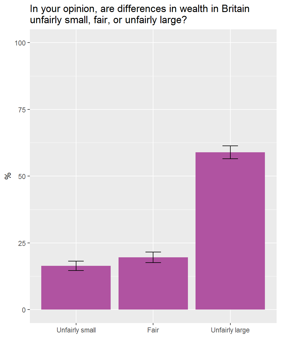
Let’s do it again for a selection of countries. First, make a function which carries out the analysis for one country:
gimme_country_results <- function(the_cntry) {
  ess9_survey %>%
    filter(cntry == the_cntry) %>%
  group_by(wltdffr_group) %>%
  summarise(prop = survey_mean(vartype = "ci")) %>%
  mutate(cntry = the_cntry)
}
Check it works for the UK:
gimme_country_results("United Kingdom")## # A tibble: 4 x 5
## wltdffr_group prop prop_low prop_upp cntry
## <fct> <dbl> <dbl> <dbl> <chr>
## 1 Unfairly small 0.164 0.146 0.181 United Kingdom
## 2 Fair 0.196 0.176 0.216 United Kingdom
## 3 Unfairly large 0.589 0.565 0.613 United Kingdom
## 4 <NA> 0.0508 0.0401 0.0615 United KingdomRun it for all the countries of interest:
conts <- c("Germany", "Spain", "France", "United Kingdom", "Italy")
euro_wealth <- map_dfr(conts, gimme_country_results)
head(euro_wealth)
## # A tibble: 6 x 5
## wltdffr_group prop prop_low prop_upp cntry
## <fct> <dbl> <dbl> <dbl> <chr>
## 1 Unfairly small 0.261 0.241 0.281 Germany
## 2 Fair 0.121 0.106 0.135 Germany
## 3 Unfairly large 0.557 0.535 0.579 Germany
## 4 <NA> 0.0619 0.0508 0.0730 Germany
## 5 Unfairly small 0.212 0.192 0.232 Spain
## 6 Fair 0.0698 0.0575 0.0822 SpainNext, try a plot:
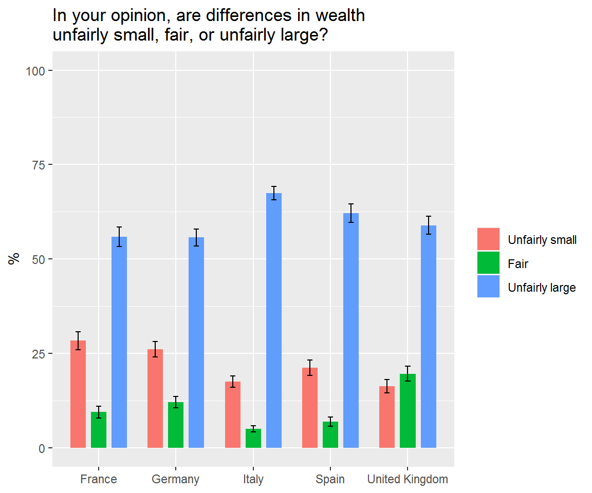
euro_wealth %>%
  filter(!is.na(wltdffr_group)) %>%
  ggplot(aes(x = cntry,
             y = prop*100,
             ymin = prop_low*100,
             ymax = prop_upp*100,
             fill = wltdffr_group)) +
  geom_col(position = position_dodge(width = .8), width = 0.6) +
  geom_errorbar(position=position_dodge(width = .8),
                colour="black",
                width = 0.2) +
  ylim(0,100) +
  labs(y = "%", x = NULL,
       title = "In your opinion, are differences in wealth\nunfairly small, fair, or unfairly large?",
       fill = NULL)